Finding the ground state of a dual-species Bose-Einstein condensate

This example demonstrates the calculation of the ground state of a dual-species Bose-Einstein condensate. We use the Gross-Pitaevskii equation (GPE) to describe the dynamics of the two wavefunctions and perform an imaginary time evolution using the split-step method to find the ground state. For further details and for the specific configuration used in this example, refer to: Pichery et al., AVS Quantum Sci. 5, 044401 (2023); doi: 10.1116/5.0163850.

Since this example uses three dimensions it requires high performance and we recommend running it on a GPU in the examplescuda environment. For this reason it is also written in JAX with jax.lax.scan.

Imports and setup

Import basic libraries and enable float64 precision types in JAX.

from functools import reduce
from typing import (
    Dict, Iterable, Any, Optional, Tuple, TypedDict
)
import os

from scipy import constants # type: ignore
import numpy as np
import jax.numpy as jnp
from jax import config
import fftarray as fa

# Enable double float precision for jax
config.update("jax_enable_x64", True)

Physical setup

Define the potential between the two interacting atomic species and basic physical constants.

# --------------------
# Physical constants
# --------------------

hbar: float = constants.hbar
a_0: float = constants.physical_constants['Bohr radius'][0]
kb: float = constants.Boltzmann

# coupling constant (used in GPE)
def coupling_fun(m_red: float, a: float) -> float:
    return 2 * np.pi * hbar**2 * a / m_red

# Rubidium 87
m_rb87: float = 86.909 * constants.atomic_mass # The atom's mass in kg.
a_rb87: float = 98 * a_0 # s-wave scattering length
# coupling constant (used in GPE)
coupling_rb87: float = coupling_fun(0.5*m_rb87, a_rb87)

# Potassium 41
m_k41: float = 40.962 * constants.atomic_mass # The atom's mass in kg.
a_k41: float = 60 * a_0 # s-wave scattering length
# coupling constant (used in GPE)
coupling_k41: float = coupling_fun(0.5*m_k41, a_k41)

# Interspecies interaction
a_rb87_k41: float = 165.3 * a_0
reduced_mass_rb87_k41 = m_rb87 * m_k41 / (m_rb87 + m_k41)
# coupling constant (used in GPE)
coupling_rb87_k41: float = coupling_fun(reduced_mass_rb87_k41, a_rb87_k41)


# Define dual species GPE potentials
def gpe_potential_two_species(
    psi_pos_sq_1: fa.Array,
    psi_pos_sq_2: fa.Array,
    coupling_constant_1: float,
    coupling_constant_12: float,
    trap_potential_1: fa.Array,
    num_atoms_1: float,
    num_atoms_2: float,
) -> fa.Array:
    """
    Calculate the 2-species GPE potential for species number 1.
    This does not include the energies that only depend on the other species.
    This does not include the kinetic energy.
    """
    self_interaction = num_atoms_1 * coupling_constant_1 * psi_pos_sq_1
    interaction_12 = num_atoms_2 * coupling_constant_12 * psi_pos_sq_2
    return self_interaction + interaction_12 + trap_potential_1

Quantum mechanics helpers

These functionalities can also be found in the matterwave library.

Get ground state of quantum harmonic oscillator.

This function creates an fa.Array from the given coordinates and trap frequencies.

def ground_state_ho(
    mass: float,
    omegas: Iterable[float],
    pos_coords: Iterable[fa.Array],
) -> fa.Array:
    psi = fa.full([], "pos", 1.0, xp=jnp)
    for omega, pos_1d in zip(omegas, pos_coords, strict=True):
        psi = (
            psi * (omega / (np.pi*hbar))**(1/4)
            * fa.exp(-mass * omega * (pos_1d**2)/(2*hbar))
        )
    norm = fa.integrate(fa.abs(psi)**2)
    return psi / fa.sqrt(norm)

Imaginary time propagation

A basic implementation of imaginary time propagation using the split-step method.

def split_step_imaginary_time(
    psi: fa.Array,
    V: fa.Array,
    dt: float,
    mass: float,
) -> fa.Array:
    """Perform an imaginary time split-step of second order in VPV configuration."""

    # Calculate half step imaginary time potential propagator
    V_prop = fa.exp((-0.5*dt / hbar) * V)
    # Calculate full step imaginary time kinetic propagator (k_sq = kx^2 + ky^2 + kz^2)
    k_sq = reduce(lambda a,b: a+b, [
        (2*np.pi * fa.coords_from_dim(dim, "freq", xp=jnp, dtype=jnp.float64))**2
        for dim in psi.dims
    ])
    T_prop = fa.exp(-dt * hbar * k_sq / (2*mass))

    # Apply half potential propagator
    psi = V_prop * psi.into_space("pos")

    # Apply full kinetic propagator
    psi = T_prop * psi.into_space("freq")

    # Apply half potential propagator
    psi = V_prop * psi.into_space("pos")

    # Normalize after step
    state_norm = fa.integrate(fa.abs(psi)**2)
    psi = psi / fa.sqrt(state_norm)

    return psi

Energy computation

Compute the kinetic and potential energy of a given wave function.

def get_e_kin(
    psi: fa.Array,
    mass: float,
):
    """Calculate the kinetic energy of the wavefunction."""
    # Calculate k^2 = (2πf)^2
    ksq = reduce(lambda a,b: a+b, [
        (2*np.pi * fa.coords_from_dim(dim, "freq", xp=jnp, dtype=jnp.float64))**2
        for dim in psi.dims
    ])

    post_factor = hbar**2 / (2*mass)

    # Calculate |ψ(f)|^2
    wf_abs_sq = fa.abs(psi.into_space("freq"))**2

    # Calculate E_kin = <ψ|(hbar*k)^2/2m|ψ> = ∫|ψ(f)|^2 * k^2 df * hbar^2 / (2m)
    return fa.integrate(wf_abs_sq * ksq).values("freq") * post_factor

def get_e_pot(
        psi: fa.Array,
        V: fa.Array,
    ):
    return fa.integrate(
        fa.abs(psi.into_space("pos"))**2 * V,
        dtype="float64"
    ).values("pos") / (kb * 1e-6)

Definition of the state initialization and the step function

The simulation loop is in this example written with jax.lax.scan in order to achieve high performance, especially on a GPU.

calc_ground_state_two_species sets up the domain and the physical problem and then runs imaginary_time_step_dual_species in a loop to execute the optimization.

from jax.lax import scan
# Register fftarray pytree nodes for JAX
try:
    fa.jax_register_pytree_nodes()
except ValueError:
    print(
        "JAX pytree nodes registration failed. " \
        "Probably due to being already registered."
    )

class DualSpeciesProperties(TypedDict):
    psi_rb87: fa.Array
    psi_k41: fa.Array
    rb_potential: fa.Array
    k_potential: fa.Array
    num_atoms_rb87: float
    num_atoms_k41: float


def calc_ground_state_two_species(
    N_iter: int,
    plot_dir: Optional[str] = None,
) -> Tuple[DualSpeciesProperties, Dict[str, Any]]:

    if plot_dir and not os.path.exists(plot_dir):
        os.makedirs(plot_dir)

    dt_list = np.full(N_iter, 5e-7)

    # Number of atoms
    num_atoms_rb87 = 43900
    num_atoms_k41 = 14400

    rb_omega_x = 2*np.pi * 24.8 # rad/s
    rb_omega_y = 2*np.pi * 378.3 # rad/s
    rb_omega_z = 2*np.pi * 384.0 # rad/s

    k_omega_x = rb_omega_x * np.sqrt(m_rb87/m_k41)
    k_omega_y = rb_omega_y * np.sqrt(m_rb87/m_k41)
    k_omega_z = rb_omega_z * np.sqrt(m_rb87/m_k41)

    # --------------------
    # fftarray definitions
    # --------------------

    # Define dimensions

    x_dim = fa.dim_from_constraints(
        "x",
        pos_extent=400e-6,
        n=2**9,
        freq_middle=0.,
        pos_middle=0.,
        dynamically_traced_coords=False,
    )

    y_dim = fa.dim_from_constraints(
        "y",
        pos_extent=50e-6,
        n=2**8,
        freq_middle=0.,
        pos_middle=0.,
        dynamically_traced_coords=False,
    )

    z_dim = fa.dim_from_constraints(
        "z",
        pos_extent=50e-6,
        n=2**7,
        freq_middle=0.,
        pos_middle=0.,
        dynamically_traced_coords=False,
    )

    # Define 1d arrays
    x: fa.Array = fa.coords_from_dim(x_dim, "pos", xp=jnp, dtype=jnp.float64)
    y: fa.Array = fa.coords_from_dim(y_dim, "pos", xp=jnp, dtype=jnp.float64)
    z: fa.Array = fa.coords_from_dim(z_dim, "pos", xp=jnp, dtype=jnp.float64)

    # Define 3d arrays for potential
    rb_potential = 0.5 * m_rb87 * (
        rb_omega_x**2 * x**2
        + rb_omega_y**2 * y**2
        + rb_omega_z**2 * z**2
    )
    k_potential = 0.5 * m_k41 * (
        k_omega_x**2 * x**2
        + k_omega_y**2 * y**2
        + k_omega_z**2 * z**2
    )

    # Define 3d arrays for initial wavefunction
    init_psi = fa.full((x_dim, y_dim, z_dim), "pos", 1, xp=jnp, dtype=jnp.float64)
    state_norm = fa.integrate(fa.abs(init_psi)**2)

    init_psi_rb = init_psi / fa.sqrt(state_norm)
    init_psi_k = init_psi / fa.sqrt(state_norm)

    # When using jax.lax.scan, the input fa.Array must have the same properties as
    # the output one. As the scanned method imaginary_time_step_dual_species
    # returns the fa.Array with space="pos" and factors_applied=False,
    # we transform the input state accordingly.
    init_psi_rb = init_psi_rb.into_space("pos").into_factors_applied(False)
    init_psi_k = init_psi_k.into_space("pos").into_factors_applied(False)

    init_properties: DualSpeciesProperties = {
        "psi_rb87": init_psi_rb,
        "psi_k41": init_psi_k,
        "rb_potential": rb_potential,
        "k_potential": k_potential,
        "num_atoms_rb87": num_atoms_rb87,
        "num_atoms_k41": num_atoms_k41
    }

    res: Tuple[DualSpeciesProperties, Dict[str, Any]] = scan(
        f=imaginary_time_step_dual_species, # type: ignore
        init=init_properties,
        xs=dt_list,
    )

    return res



def imaginary_time_step_dual_species(
    properties: DualSpeciesProperties,
    dt: float,
) -> Tuple[DualSpeciesProperties, Dict[str, float]]:
    """
    Perform a single imaginary time step for the dual species GPE.
    Additionally, calculate all relevant energies.
    The states are returned in position space.
    """

    psi_rb87 = properties["psi_rb87"]
    psi_k41 = properties["psi_k41"]
    rb_potential = properties["rb_potential"]
    k_potential = properties["k_potential"]
    num_atoms_rb87 = properties["num_atoms_rb87"]
    num_atoms_k41 = properties["num_atoms_k41"]

    ## Calculate the potential energy operators (used for split-step and plots)
    psi_rb87 = psi_rb87.into_space("pos")
    psi_k41 = psi_k41.into_space("pos")

    psi_pos_sq_rb87 = fa.abs(psi_rb87)**2
    psi_pos_sq_k41 = fa.abs(psi_k41)**2

    self_interaction_rb87 = num_atoms_rb87 * coupling_rb87 * psi_pos_sq_rb87
    interaction_rb87_k41 = num_atoms_k41 * coupling_rb87_k41 * psi_pos_sq_k41
    V_rb87 = self_interaction_rb87 + interaction_rb87_k41 + rb_potential

    self_interaction_k41 = num_atoms_k41 * coupling_k41 * psi_pos_sq_k41
    interaction_k41_rb87 = num_atoms_rb87 * coupling_rb87_k41 * psi_pos_sq_rb87
    V_k41 = self_interaction_k41 + interaction_k41_rb87 + k_potential

    ## Calculate energies for plotting and convergence check

    # Calculate potential energy (in µK)
    E_pot_rb87 = get_e_pot(psi_rb87, V_rb87)
    E_pot_k41 = get_e_pot(psi_k41, V_k41)

    # Calculate kinetic energy (in µK)
    E_kin_rb87: float = get_e_kin(psi_rb87, mass=m_rb87) / (kb * 1e-6)
    E_kin_k41: float = get_e_kin(psi_k41, mass=m_k41) / (kb * 1e-6)

    # Calculate the total energy
    E_tot = E_kin_rb87 + E_kin_k41 + E_pot_rb87 + E_pot_k41
    ## Imaginary time split step application

    psi_rb87 = split_step_imaginary_time(
        psi=psi_rb87,
        V=V_rb87,
        dt=dt,
        mass=m_rb87,
    )
    psi_k41 = split_step_imaginary_time(
        psi=psi_k41,
        V=V_k41,
        dt=dt,
        mass=m_k41,
    )


    return properties | {"psi_rb87": psi_rb87, "psi_k41": psi_k41}, {
        "E_kin_rb87": E_kin_rb87,
        "E_kin_k41": E_kin_k41,
        "E_pot_rb87": E_pot_rb87,
        "E_pot_k41": E_pot_k41,
        "E_tot": E_tot
    }

Run the simulation

This cell takes about 1 minute for the 5000 steps on an NVIDIA A100 GPU and may take a long time when only running on a CPU.

# Reducing the number of steps in test mode
# allows running this notebook as part of the test suite.
if os.environ.get("TEST_MODE", "False") == "True":
    N_iter=2
else:
    # This branch is taken when executed in a normal notebook
    N_iter=5000

final_properties, energies = calc_ground_state_two_species(N_iter=N_iter)

Plotting the results

import matplotlib.pyplot as plt
from bokeh.plotting import show
from bokeh.io import output_notebook
from helpers import plt_integrated_1d_densities, plt_integrated_2d_density

output_notebook(hide_banner=True)

Final state

We normalize the final states to their respective number of atoms:

rb_ground_state = (
    final_properties["psi_rb87"].into_space("pos")
    * np.sqrt(final_properties["num_atoms_rb87"])
)
k_ground_state = (
    final_properties["psi_k41"].into_space("pos")
    * np.sqrt(final_properties["num_atoms_k41"])
)

Integrating in the \(z\) dimension yields a two dimensional plot per species and space. Use the zoom tool in the plots to zoom in on the details of the simulation.

show(
    plt_integrated_2d_density(
        rb_ground_state,
        red_dim_name="z",
        data_name="Rb87",
        title_prefix="N",
    )
)

show(
    plt_integrated_2d_density(
        k_ground_state,
        red_dim_name="z",
        data_name="K41",
        title_prefix="N",
    )
)

Integrating in \(y\) and \(z\) yields allows us to plot the probability densities of both species:

show(
    plt_integrated_1d_densities(
        arrs={"Rb87": rb_ground_state, "K41": k_ground_state},
        red_dim_names=["y", "z"],
        # Zoom in a bit to see the spatial structures better.
        x_range_pos=(-4e-5, +4e-5),
        x_range_freq=(-1e5, +1e5),
        y_label_prefix="N",
    )
)

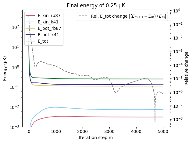
Energies as a function of iteration steps

COLORS = ["#CC6677", "#88CCEE", "#DDCC77", "#332288", "#117733"]

fig, ax1 = plt.subplots()

ax1.plot(energies["E_kin_rb87"], label="E_kin_rb87", color=COLORS[0])
ax1.plot(energies["E_kin_k41"], label="E_kin_k41", color=COLORS[1])
ax1.plot(energies["E_pot_rb87"], label="E_pot_rb87", color=COLORS[2])
ax1.plot(energies["E_pot_k41"], label="E_pot_k41", color=COLORS[3])
ax1.plot(energies["E_tot"], label="E_tot", color=COLORS[4])

ax1.set_title(f"Final energy of {energies['E_tot'][-1]:.2f} µK")
ax1.set_xlabel("Iteration step m")
ax1.set_ylabel("Energy (µK)")
ax1.set_yscale("log")
ax1.set_ylim(bottom=1e-3)
ax1.legend(loc="upper left")

ax2 = ax1.twinx()
relative_change = np.abs(np.diff(energies["E_tot"]) / energies["E_tot"][:-1])
ax2.plot(
    np.arange(1, len(energies["E_tot"])),
    relative_change,
    color="gray",
    linestyle="--",
    label=r"Rel. E_tot change $|(E_{m+1}-E_m) \:/ \: E_{m}|$",
)
ax2.set_ylabel("Relative change")
ax2.set_yscale("log")
ax2.legend(loc="upper right")

plt.tight_layout()